Bits vs Qubits: The Real Difference Between Classical and Quantum Information

When comparing a classical bit to a quantum bit (qubit), the distinction is not simply about processing speed. The fundamental difference lies in information density and computational mechanics. While standard computers rely on linear, deterministic switches to process data one step at a time, quantum computers leverage multi-dimensional probability to evaluate vast computational landscapes simultaneously.

Every quantum computing explainer tells you qubits are better because of superposition. Almost none of them tell you why that actually matters or when it doesn’t.

That gap is exactly what this article closes.

The Classical Bit: A Definite Answer, Always

A classical bit is the fundamental unit of information in every computer you’ve ever used. It exists in one of two states: 0 or 1. On or off. True or false. There’s no ambiguity, no in-between, no probability involved.

Physically, a bit is implemented as a transistor a tiny switch that’s either open (0) or closed (1). Modern processors contain billions of them, switching states billions of times per second.

That simplicity is a feature, not a limitation. Classical bits are:

• Stable — a bit holds its state until something changes it
• Readable — you can check a bit’s value without disturbing it
• Scalable — billions of bits fit on a chip the size of a fingernail
• Reliable — error rates in classical memory are vanishingly small

Eight bits form a byte. A byte can represent 256 distinct values. Scale that up and you get the entire information infrastructure of the modern world every file, message, image, and video encoded in sequences of 0s and 1s.

Classical bits process information through logic gates: AND, OR, NOT, NAND. Chain enough gates together and you can compute anything computable. That’s not a small thing. Most of what you’d ever want a computer to do falls inside that boundary.

Qubits: Quantum Information With a Twist

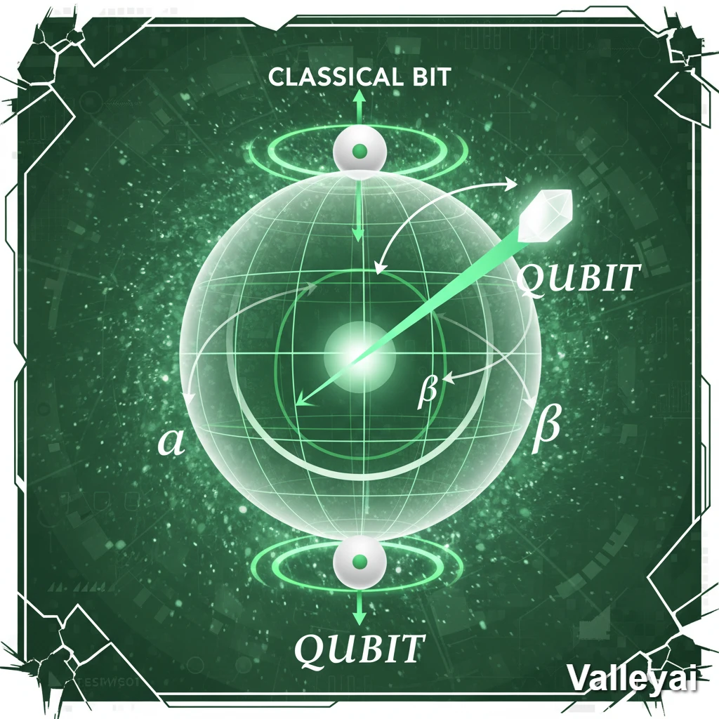
A qubit short for quantum bit is the fundamental unit of information in a quantum computer. Like a classical bit, it has two basis states: |0⟩ and |1⟩. Unlike a classical bit, it doesn’t have to be in one of them.

Before measurement, a qubit can exist in a superposition of both states simultaneously. Mathematically, its state is described as:

|ψ⟩ = α|0⟩ + β|1⟩

Where α and β are probability amplitudes complex numbers whose squared magnitudes give the probability of measuring 0 or 1 respectively. The constraint: |α|² + |β|² = 1.

The Bloch sphere is the standard visualization for this: imagine a sphere where the north pole is |0⟩ and the south pole is |1⟩. A classical bit can only be at one of those poles. A qubit can point anywhere on the surface representing a continuum of possible states.

Qubits are physically realized as two-state quantum systems. The most common implementations:

Implementation	Physical Basis	Used By
Superconducting qubits	Microwave-controlled superconducting circuits at near absolute zero	IBM, Google, Rigetti
Trapped ion qubits	Individual ions suspended in electromagnetic fields	IonQ, Honeywell
Photonic qubits	Polarization or path states of individual photons	PsiQuantum, Xanadu

Each implementation represents a different tradeoff between coherence time, gate fidelity, and scalability. There’s no consensus winner and that uncertainty reflects how early-stage this field still is.

Side-by-Side: What Actually Differs

Before going deeper into mechanisms, here’s the structural contrast:

Property	Classical Bit	Qubit
Possible states	0 or 1 (definite)	Superposition of 0 and 1 (probabilistic)
State during computation	Fixed and readable	Fragile; reading destroys superposition
Correlation between units	Independent	Can be entangled (correlated quantum states)
Error rate	Extremely low	High — requires error correction
Physical stability	Stable at room temperature	Requires extreme isolation (often near 0 Kelvin)
Information per unit	1 bit	1 qubit (but encodes amplitude information)
Processing mechanism	Logic gates (AND, OR, NOT)	Quantum gates (unitary transformations)
Scalability	Mature — billions per chip	Early-stage — hundreds to thousands, with errors

The table makes it look like qubits are simply better. They’re not. They’re different and that difference only matters for specific problems.

Superposition Isn’t Magic — Here’s the Actual Mechanism

Most introductions to qubits describe superposition as “existing in both states at once,” which sounds profound but misses the computational point entirely. The Reddit question that’s ranking in Google for this topic is essentially asking: what does that actually mean for computation? It’s a fair question, and most explainers dodge it.

Here’s the mechanism that actually matters:

Step 1: Superposition Creates a Parallel Exploration Space

When n qubits are placed in superposition, the system can represent 2^n states simultaneously. Two qubits: 4 states. Ten qubits: 1,024 states. 300 qubits: more states than there are atoms in the observable universe.

A classical computer exploring 2^n states must check them sequentially. A quantum computer holds all 2^n states in superposition at once. That’s the parallel exploration advantage but it’s not the whole story.

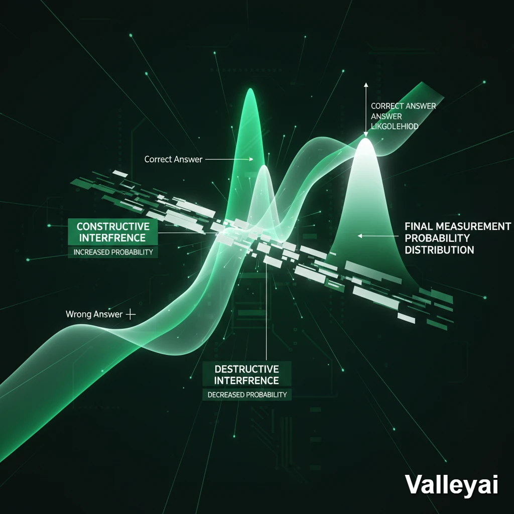
Step 2: Quantum Interference Filters the Answer

Here’s what most explanations skip: you can’t just “read” all 2^n states at once. Measurement collapses the superposition to a single state randomly. If you measured immediately after superposition, you’d get a random answer, no better than guessing.

The real computational work happens through quantum interference. Quantum algorithms are designed to manipulate probability amplitudes so that:

• Amplitudes corresponding to wrong answers cancel each other out (destructive interference)
• Amplitudes corresponding to correct answers reinforce each other (constructive interference)

By the time you measure, the correct answer has high probability. Wrong answers have near-zero probability. Measurement becomes reliable, not random.

Step 3: Measurement Extracts the Result

Measurement collapses the qubit’s superposition to a definite state: 0 or 1. The probability of each outcome is determined by the amplitude manipulation in Step 2. A well-designed quantum algorithm makes the correct answer overwhelmingly probable.

This is why quantum algorithm design is hard. You’re not programming a computer to compute an answer you’re programming it to set up an interference pattern so that measurement yields the answer with high probability. That’s a fundamentally different programming paradigm.

Designing an algorithm that sets up the right interference pattern is the genuinely difficult part of quantum computing. The superposition is easy. The interference engineering is where the expertise lives.

Entanglement: Correlated Quantum States Across Space

Entanglement is the second major quantum property that distinguishes qubits from classical bits. Two qubits are entangled when their quantum states are correlated measuring one instantly determines the state of the other, regardless of physical separation.

A classical analogy that almost works: imagine writing “0” on one card and “1” on another, sealing them in envelopes, and mailing them to opposite sides of the world. When you open yours and see “0,” you instantly know the other is “1.” That’s correlation, not entanglement.

The quantum version is stranger. Before measurement, neither qubit has a definite value. Measurement of one qubit creates the correlated outcome in both. The correlation isn’t pre written it emerges from measurement.

For computation, entanglement matters because it allows quantum gates to operate on correlated qubit systems. Operations on one qubit affect the state of its entangled partner. This enables quantum algorithms to explore correlated solution spaces that classical bits simply cannot represent efficiently.

Bell states are the simplest examples of entangled qubit pairs the four maximally entangled two-qubit states that form the foundation of quantum information theory.

Exponential Scaling: The Number That Changes Everything

With n classical bits, you can represent any one of 2^n possible values at a given moment. To process all 2^n values, you process them one at a time — sequentially.

With n qubits in superposition, all 2^n states are represented simultaneously in the quantum state of the system. The system doesn’t process them one at a time. It evolves all of them in parallel through quantum gate operations.

That’s the exponential advantage and it’s real, but it comes with a catch.

You can only extract one measurement outcome. The art of quantum computing is designing the algorithm so that the one outcome you extract is the one you wanted. This is why quantum algorithms aren’t universally faster they only outperform classical algorithms for specific problem structures where interference can be exploited effectively.

For problems without that structure, quantum parallelism provides no advantage. A quantum computer sorting a list of numbers isn’t faster than a classical computer. The interference pattern required to make sorting work on a quantum computer doesn’t exist in a useful form.

Where Qubits Genuinely Win: Specific Problem Classes

Qubits outperform classical bits for a narrow but important set of problem types. Not because they’re generally faster, but because specific quantum algorithms exploit superposition and interference in ways that classical algorithms cannot match.

Factorization (Shor’s Algorithm)
Shor’s algorithm factors large integers in polynomial time on a quantum computer. The best classical algorithms require exponential time. For a 2048-bit number the kind used in RSA encryption a classical computer would take longer than the age of the universe. A sufficiently powerful quantum computer could factor it in hours.

Database Search (Grover’s Algorithm)
Grover’s algorithm searches an unsorted database of N items in O(√N) time. Classical search requires O(N) time. That’s a quadratic speedup meaningful for large databases, though not the exponential leap that Shor’s algorithm provides.

Quantum Simulation
Simulating quantum systems molecules, chemical reactions, materials requires classical computers to track an exponentially growing number of quantum states. Quantum computers simulate quantum systems naturally, using fewer resources. This is the application most physicists and chemists are watching closely.

Optimization Problems
Certain optimization problems logistics, financial modeling, drug discovery have solution spaces too large for classical exhaustive search. Quantum algorithms like the Quantum Approximate Optimization Algorithm (QAOA) may provide speedups, though this remains an active research area.

The Qubit Reality: Decoherence and the NISQ Ceiling

Here’s the part most explainers skip because it complicates the narrative.

Qubits are extraordinarily fragile. Any interaction with the environment heat, vibration, electromagnetic interference, even cosmic rays can disrupt the quantum state. This disruption is called decoherence, and it’s the defining engineering challenge of quantum computing.

Current superconducting qubits maintain coherence for microseconds to milliseconds. In that window, you must initialize the qubit, perform all quantum gate operations, and extract the measurement. A single quantum gate takes nanoseconds so the margin is tight but workable, for small circuits. As circuits grow deeper (more gate operations), decoherence accumulates and errors multiply.

The error rates in current quantum hardware are orders of magnitude higher than classical bits. A classical bit flip error is a rare event. A qubit error can happen on every gate operation, at rates between 0.1% and 1% per gate.

The error correction paradox:

Quantum error correction (QEC) can fix these errors but it requires encoding a single logical qubit across multiple physical qubits. Current estimates suggest you need 1,000 to 10,000 physical qubits to produce one reliable logical qubit.

So when IBM announces a 1,000-qubit processor, that’s 1,000 physical qubits which might encode fewer than 10 reliable logical qubits for fault-tolerant computation. The gap between physical qubit count and useful logical qubit count is the current scaling wall.

This is the NISQ era Noisy Intermediate-Scale Quantum the term coined by physicist John Preskill of Caltech to describe the current phase of quantum computing: systems with 50 to 1,000 qubits, high error rates, and no fault-tolerant error correction.

In the NISQ era, quantum computers can demonstrate interesting results on carefully chosen problems. They cannot yet reliably outperform classical computers on practical, real-world tasks.

Where Classical Bits Still Win — Which Is Most Places

If you’re sorting a list, running a database query, compressing a video, serving a web page, training a neural network, or doing anything that most software does classical bits are faster, cheaper, more reliable, and more practical. Full stop.

Quantum computers aren’t general-purpose replacements for classical computers. They’re specialized accelerators for a narrow class of problems where quantum algorithms provide a structural advantage. The analogy isn’t “quantum computers vs. classical computers” it’s closer to “GPU vs. CPU.” A GPU is extraordinarily powerful for parallel matrix operations and useless for running your operating system.

Most guides on this topic present qubits as an upgrade to bits. That framing is wrong, and it leads to unrealistic expectations about what quantum computing can deliver.

The honest picture: quantum computers will likely become indispensable tools for specific domains cryptography, drug discovery, materials science, optimization at scale. For everything else, classical bits will remain the right tool for the foreseeable future.

How the Two Systems Process Information: A Workflow Comparison

Classical and quantum computation follow fundamentally different processing models.

Classical computation:

1. Input is encoded as bits (0s and 1s)
2. Logic gates (AND, OR, NOT) transform bit states deterministically
3. Output is read directly — bits are stable and readable at any point
4. Computation is sequential: one operation at a time per processor core

Quantum computation:

1. Input is encoded into qubit states (initialization)
2. Quantum gates (unitary transformations) evolve the quantum state
3. Superposition and entanglement allow parallel evolution of 2^n states
4. Interference is engineered to amplify correct outcomes
5. Measurement collapses the quantum state to extract the result
6. Due to probabilistic measurement, algorithms often run multiple times to confirm results

The fundamental architectural difference: classical computation is deterministic at every step. Quantum computation is probabilistic until measurement. The algorithm’s job is to make that probability as close to certainty as possible.

Quantum Volume: How We Measure Qubit System Capability

Raw qubit count is a misleading metric for quantum computer performance. IBM developed Quantum Volume as a more meaningful benchmark a single number that accounts for qubit count, connectivity, gate fidelity, and error rates together.

A system with 50 high-quality, well-connected qubits may have higher Quantum Volume than a system with 100 noisy, poorly connected qubits. The metric captures the practical computational power of the system, not just its headline number.

This matters when evaluating announcements about quantum computing milestones. “1,000 qubits” sounds more impressive than it often is.

Final Thoughts

The gap between what qubits can theoretically do and what they currently do is the defining tension in quantum computing. Understanding that gap not just the superposition headline is what separates a realistic view of this technology from the hype cycle. The bits vs qubits question isn’t really about which is better. It’s about understanding two fundamentally different computational paradigms, each suited to different problems, operating at different points on the maturity curve. Knowing which tool fits which problem is the skill that will matter most as quantum systems scale.

---

Frequently Asked Questions