How Does Speech Recognition Work? From Sound Waves to Words on Screen

What speech recognition answers?

Captions appear on screen while a person is still talking. A voice assistant answers a question spoken across the room. A doctor dictates notes and the words land in the record without a keyboard.

Every one of these moments runs on the same system. Speech recognition, also called automatic speech recognition or ASR, turns spoken audio into written text. It answers one question: which words were spoken.

That question is narrower than it sounds. Speech recognition does not decide who spoke. Identifying the speaker is a separate task called voice recognition. A system can transcribe a stranger perfectly without knowing their name, and it can recognize a familiar voice without understanding a word they said. Mixing the two up is the most common confusion about the field.

Match the engine to your audio, not to the leaderboard. A leaderboard number comes from clean read speech. Your audio is a phone call, a meeting room, a car. The gap between those two settings is the whole buying decision, and the test measures it on one sentence.

The same pipeline sits behind live captions, voice assistants, dictation software, call centre transcripts, and medical notes. The words change, the stages do not.

The test: one sentence, four conditions

A claim about accuracy means little without the test behind it. So a test was run. The test sentence was “Schedule the meeting for Tuesday at three, and remind Maya to bring the report on wind turbines.” Whisper’s base model transcribed it four ways: clean, with white noise mixed in, sped up, and in a second voice. A fifth clip tested a sentence built to trap the language model.

Transcribed with Whisper’s base model on 11 November 2026. The audio was synthesized with a text-to-speech voice, the ground truth was known in advance, and each clip ran once.

Condition	Words misheard	Words-only WER	What happened
Clean, first voice	0 of 17	0.0%	Word-perfect; one comma dropped
White noise, 9 dB SNR	2 of 17	17.6%	“Wind turbines” became “winter bus”
1.3x speed	0 of 17	5.9%	“Three” written as “3”
Second voice	0 of 17	5.9%	“Three” written as “3”
Homophone sentence, clean	3 of 21	28.6%	“I scream” became “Ice cream”

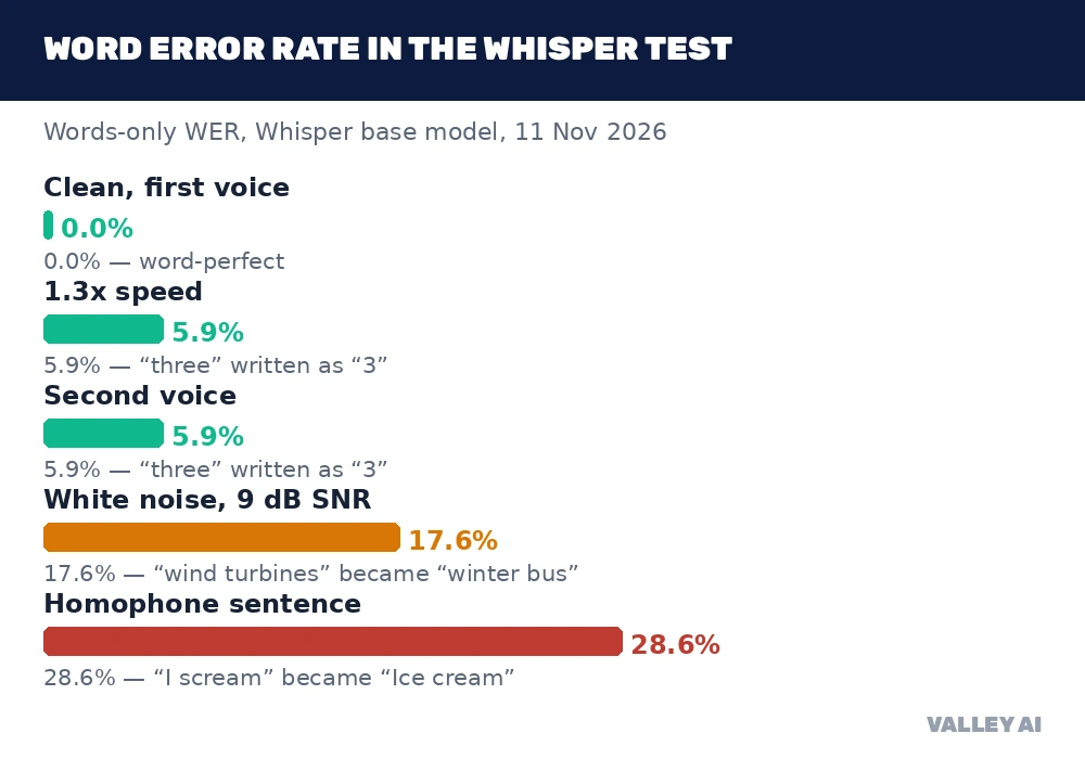
Clean speech is close to solved. The model transcribed the plain sentence word-perfect in three of the four conditions, and the only error in the fourth was a missing comma. Speed did not hurt it. A different voice did not hurt it.

Noise hurt it. At 9 decibels of signal-to-noise ratio, “wind turbines” came back as “winter bus.” Two words changed, and the sentence lost its meaning. The model’s own confidence scores marked the failure: “winter” scored 0.37 and “bus” 0.14, the lowest scores in the whole transcript.

The homophone sentence hurt it more, in clean audio. “I scream for ice cream” came back as “Ice cream for ice cream,” and “Reed” came back as “read.” The sounds fit both readings, and the language model picked the common phrase over the true one. Its confidence scores flagged both errors: “Ice” scored 0.11, “read” 0.26.

One synthetic voice reading one scripted sentence is the easiest input speech recognition ever sees. These numbers are a controlled check on one sentence. They say nothing about field conditions. Published leaderboard figures sit near 5% word error rate on clean read speech, per the Open ASR Leaderboard. The gap between that figure and your audio is the reason to test on your own recordings. Record half an hour of the audio you need transcribed, get a person to type out a few minutes of it, and score each candidate engine against that sample. No leaderboard number replaces that test.

Step one: sound becomes numbers

Sound reaches the system as a pressure wave. A microphone turns that wave into an electrical signal, and a recorder stores the signal as numbers. The first job of speech recognition is to take those numbers seriously, because everything after it works from them.

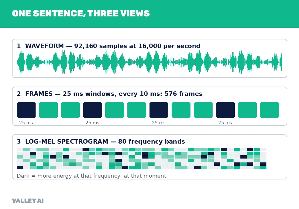
The recorder measures the wave 16,000 times per second for wideband speech. Telephone calls use 8,000. Each measurement is one sample, and the test sentence ran 5.76 seconds. That is 92,160 samples for one short sentence. Ten seconds of speech is 160,000 numbers, and a minute is close to a million.

Those samples are cut into short windows called frames. Each frame lasts 25 milliseconds, and a new one starts every 10 milliseconds, so the windows overlap. The test sentence became 576 frames. A frame is short enough that the sound inside it stays roughly steady, which is what makes the next step possible.

Frames exist because speech changes fast. A vowel can shift in a tenth of a second. A whole sentence carries too much change for one measurement, and a single sample carries too little. The frame sits between the two.

Step two: numbers become a picture of sound

A frame of raw samples is hard to read. The numbers jump up and down, and two frames of the same vowel can look different. So each frame is passed through a Fast Fourier Transform, which exposes the frequencies inside it. The result is a list of how much energy sits at each pitch.

Those frequencies are then mapped onto the mel scale, which matches human hearing. Human ears separate low pitches finely and blur high ones together, and the mel scale copies that shape. The output is a log-mel spectrogram: 80 frequency bands for each frame, with the energy in each band.

For the test sentence, that picture is 80 bands wide and 576 frames long. Every column is one 10-millisecond slice of speech. Every row is one frequency band. Dark cells hold more energy. The network reads this picture. The raw wave never reaches it.

An older feature, the mel-frequency cepstral coefficient, or MFCC, did the same job from the 1980s through the 2010s. Modern end-to-end systems skip it and feed the log-mel spectrogram straight to the network. The picture carries the same information with less processing in between.

This is the step where the audio stops being sound and starts being data the model can compare. Two recordings of the same word produce similar pictures. Two different words produce different ones.

Step three: the network guesses words

The spectrogram goes into an encoder, a neural network that reads the whole picture at once and turns each frame into a vector that carries context from the frames around it. Most current encoders are built on the transformer, the same architecture behind large language models. The decoder then turns those vectors into text, one token at a time.

Three decoder designs dominate the field. CTC lines each frame up with a letter and collapses repeats. RNN-T emits words as the audio arrives, which suits live captions. Attention decoders look back across the whole sentence before choosing each word. Whisper uses an attention decoder.

The decoder does not pick one word and move on. It keeps several candidate sentences alive at once, scores each against the audio and the language model, and drops the ones that stop making sense. This is beam search, and it works like a shortlist that narrows as more sound arrives.

Confidence scores come with every word. In the clean test run, “Schedule” scored 0.64, “three” 0.36, and “wind” 0.65. The words it got wrong scored lower still. Low-confidence words are the ones to check in any transcript, because the model already knows where it is guessing.

Why does it write “3” when I said “three”? The transcript is formatted for reading. It does not try to match the sounds. A step called inverse text normalisation turns spoken numbers into digits, so “two fifteen” becomes “215” and “fourth” becomes “4th.” The sounds were right. The spelling followed a formatting rule.

OpenAI published Whisper in 2022. The model was trained on labeled examples: 680,000 hours of audio paired with transcripts, covering about 100 languages. The training data is why it handles accents and background noise better than the models that came before it. The same data explains the failures: the cases the data covered least are the cases it handles worst.

Where it goes wrong

Word error rate, the standard accuracy metric defined in Jurafsky and Martin’s Speech and Language Processing, counts three kinds of mistakes. A substitution swaps one word for another. A deletion drops a word. An insertion adds a word nobody said. The test produced substitutions and a deletion. It produced no insertion, which is the rarest of the three in a short clean clip.

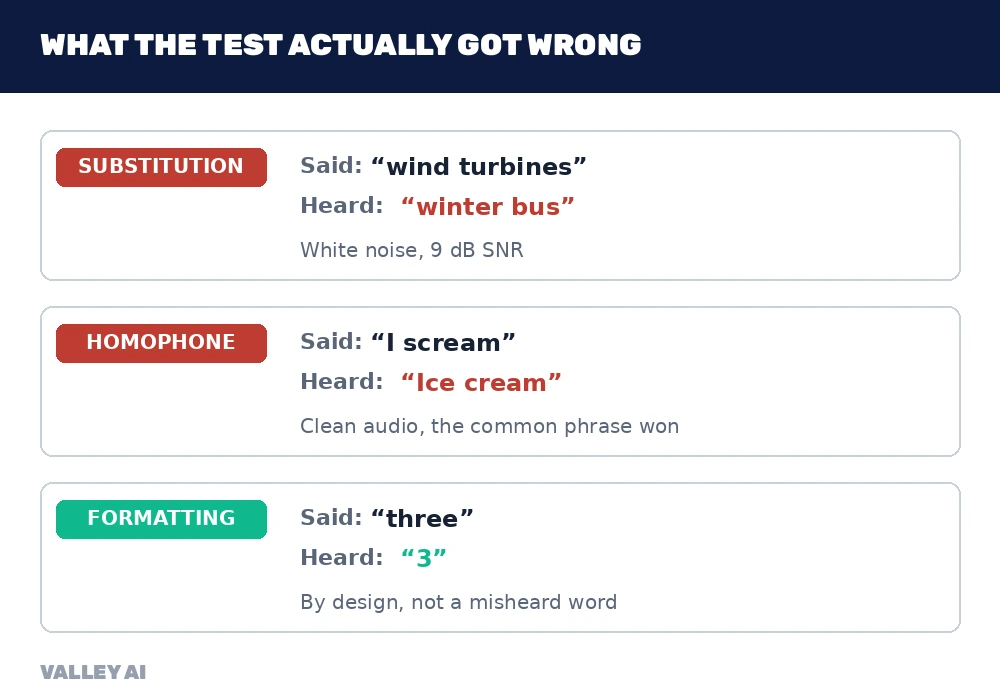
Substitution is the error that changes meaning. Noise caused the one in this test, and the mechanism is simple to state. Noise masks the fine detail that separates similar sounds, and the language model fills the gap with the more common phrase. “Winter bus” is a phrase English uses. “Wind turbines” needs the context of the report to win, and the model had no report.

Why did noise turn “wind turbines” into “winter bus”? The noise sat at 9 decibels of signal-to-noise ratio, loud enough to flatten the high-frequency detail that separates “d” from “t” and the tail of one word from the start of the next. With the sound blurred, the language model chose the phrase it had seen more often. The confidence scores confirm it: “winter” scored 0.37, “bus” 0.14, against 0.98 or higher for the words around them.

Homophones break the system in clean audio, where noise cannot take the blame. “I scream” and “ice cream” sound identical. “Reed” and “read” sound identical. The model can only use context. Context points to the likely reading, and the likely reading can be wrong. The classic classroom example is “recognize speech” against “wreck a nice beach,” and the test sentence showed the same failure with real numbers.

Accents raise the error rate further. LearnHowToScience lists accent error rates running 2 to 5 times higher than for the best-covered accent. The cause is the training data: a model hears the accents in its data most, and the rest less.

The strangest failure is hallucination. A neural model can invent words during long silences or heavy noise, writing sentences nobody spoke. Reson8’s review names it as a live failure mode, and it is the reason a transcript of a noisy meeting needs a human check before it goes into a record.

LearnHowToScience puts the sharp drop below 5 decibels of signal-to-noise ratio. That number is a practical line: a recording quieter than the room around it is a recording the model will guess at.

Streaming or batch, on-device or cloud

The pipeline is the same in every product. What changes is where it runs and when the text appears. Those two choices decide the accuracy, the delay, and the privacy of the result.

Choice	What it is	Pick it when	What it costs
Streaming	Text appears while the person is still speaking	Live captions, voice assistants	Accuracy; the model guesses with less context
Batch	The whole recording is processed at once	Meeting notes, transcripts, dictation	Delay; the text arrives after the audio ends
On-device	A small model runs on the phone or laptop	Privacy matters, or the internet is absent	Accuracy; Whisper tiny holds 39M parameters
Cloud	A large model runs on a server	Accuracy matters most	Privacy and connection; audio leaves the device

Why do live captions lag behind the speaker? The model waits for enough sound to guess with confidence, and the audio still has to travel to the server and back. AssemblyAI reports a 307 millisecond median time-to-final for its realtime system on its own 12,460-clip benchmark. That delay is the price of text that appears while someone is still talking.

The Whisper model card lists five sizes, from tiny at 39 million parameters to large at 1.55 billion. The test used the base model at 74 million. A bigger model hears more, and it needs more hardware to run. That trade is the reason the small models live on phones and the large ones live on servers, where graphics cards carry the arithmetic.

Voice search runs the same pipeline before the query ever reaches the ranking step. The spoken words become text, and then the search engine ranks pages for that text.

Speed follows the same trade. The base model transcribed 5.76 seconds of audio in 2.7 seconds on a two-core CPU, faster than real time. Larger models on server hardware finish the same work faster, because the model runs on graphics cards.

From Audrey to Whisper

Speech recognition is more than 70 years old. The first system, Audrey, was built at Bell Labs in 1952 and recognized digits spoken by its own designers. It took a relay rack to do it, and it scored 97 to 99 percent on the voices it knew.

• 1962: IBM Shoebox recognizes 16 words, including digits and simple commands.
• 1970s-80s: Hidden Markov Models take over, with James Baker’s DRAGON thesis and Fred Jelinek’s n-gram language models.
• 1990: Dragon Dictate ships at $9,000, the first consumer dictation product.
• 1997: Dragon NaturallySpeaking brings continuous dictation to the desktop.
• 2008: Google Voice Search launches, trained on 230 billion words of search queries.
• 2011: Siri puts speech recognition in every iPhone.
• 2012: Deep learning enters the field with Hinton’s acoustic models.
• 2014: Baidu’s Deep Speech shows an end-to-end neural network can replace the pipeline.
• 2017: Microsoft reports 5.1% word error rate on the Switchboard benchmark, matching human transcribers.
• 2022: OpenAI releases Whisper, trained on 680,000 hours.

Error rates fell as the data grew. The Stanford AI Index puts speech error rates at 43% in 2013 and below 5% in 2025. The curve is the story of the field: more audio, more transcripts, better models, and the same pipeline underneath.

The history matters because it sets the expectation. Whisper and its rivals are the latest step in a long line, refining an old idea. The failures in the test are the failures the field has carried for decades: noise, accents, and words that sound alike.

Pick the setup that fits your audio

Start from the audio. The model follows from it. Clean recordings of one speaker in a quiet room run well on a small on-device model. Noisy recordings, strong accents, and long meetings need a large cloud model, and they still need a human check on the low-confidence words.

If the text must appear live, pick streaming and accept the delay and the lower accuracy. If it can wait, pick batch and get the better transcript.

Record a sample of the speech you need transcribed, run it through two engines, and compare the word error rates. The engine that wins on your audio is the one to buy.

Frequently asked questions