How Does a Neural Network Work? Neurons, Weights, and a Real Training Run

A neural network earns trust one way: its error on data it never saw. A network that scores 99 percent on its training examples and 60 percent on new ones memorized the answers. A network that scores 95 percent on new examples learned the pattern. That single check separates a working model from a trick, and the mechanism behind the score is arithmetic.

The mechanism is arithmetic. A network is a stack of small computing units called neurons, wired in layers. Each neuron multiplies its inputs by numbers called weights, adds a bias, and passes the result through a bend called an activation function. Training adjusts the weights until the predictions match the right answers. Nothing inside a neuron does more than that.

What a Neural Network Is

A neural network is a machine learning model that turns inputs into predictions by passing them through layers of artificial neurons. A photo classifier takes in pixel values and returns a probability for each label. A demand forecaster takes in past sales and returns a number for next month. The shape of the input changes. The mechanism stays the same.

Inside machine learning, neural networks form the family of models that learn patterns directly from raw data, and deep learning is the name for networks with many hidden layers. Artificial intelligence is the broader goal of making computers handle tasks that need judgment. Machine learning is the branch where systems learn from data. Neural networks are one family inside that branch.

The design borrows three ideas from the brain: many simple units, weighted connections between them, and a threshold that decides whether a signal moves forward. The human brain holds about 86 billion neurons, according to a cell-counting study published in Frontiers in Human Neuroscience. Each biological neuron collects signals through its dendrites, sums them in its cell body, and fires along its axon once the total crosses a threshold.

Past that outline, the resemblance stops. Biological neurons send timed electrical spikes and rewire through life. Artificial neurons pass one continuous number that stays fixed once training ends. A neural network is a mathematical model inspired by the brain, and claims that a network thinks the way a person does go past what the math supports.

One Neuron, Worked With Real Numbers

A neuron is a small function. It multiplies each input by a weight, adds a bias, and passes the total through an activation function. Written as math, one neuron computes z = w1x1 + w2x2 + … + wnxn + b, then outputs a = f(z), where f is the activation function. Run that formula with real numbers and it looks like this:

• Inputs: 0.9, 0.2, and 0.7
• Weights: 0.5, -0.4, and 0.8, with a bias of 0.1
• Weighted sum: (0.9 x 0.5) + (0.2 x -0.4) + (0.7 x 0.8) + 0.1 = 0.45 – 0.08 + 0.56 + 0.10 = 1.03
• ReLU output: max(0, 1.03) = 1.03. The same sum through a sigmoid gives 0.737.

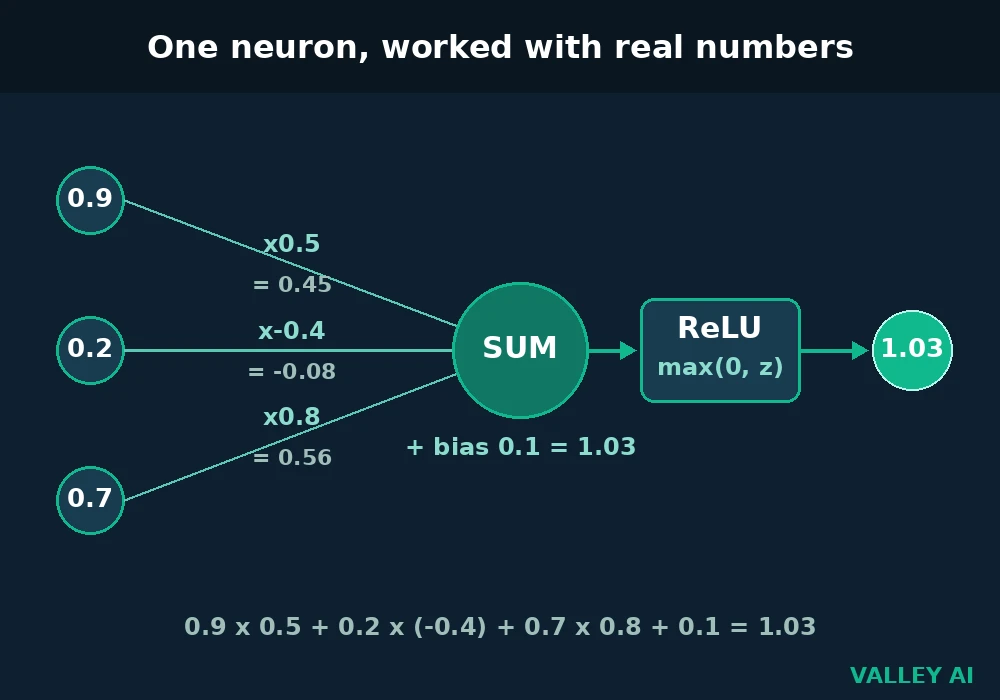
Why multiply by weights at all? A plain sum would treat every input as equal. The weight sets how much each input matters. A weight near zero tells the neuron to ignore that input. A negative weight lets an input push the output down. The bias lets a neuron produce a useful output even when every input is zero.

A weight works like a volume knob on one input. Turn it up and that input shouts. Turn it to zero and that input goes silent. Turn it negative and that input pulls the other way. Training is the process of setting every knob in the network to the position that gives the best predictions.

Layers Stack Simple Neurons Into Pattern Detectors

One neuron draws one boundary. A layer of neurons draws many at once, and a stack of layers builds on the work of the layers before it. The input layer holds the raw features. Each hidden layer reshapes what it receives into a new representation. The output layer turns the last representation into a prediction.

For images, the first hidden layer spots edges and corners. Deeper layers combine those edges into shapes, then into parts, then into whole objects. The network is never told what an edge is. The layers settle into that division because it is the arrangement that shrinks the error fastest.

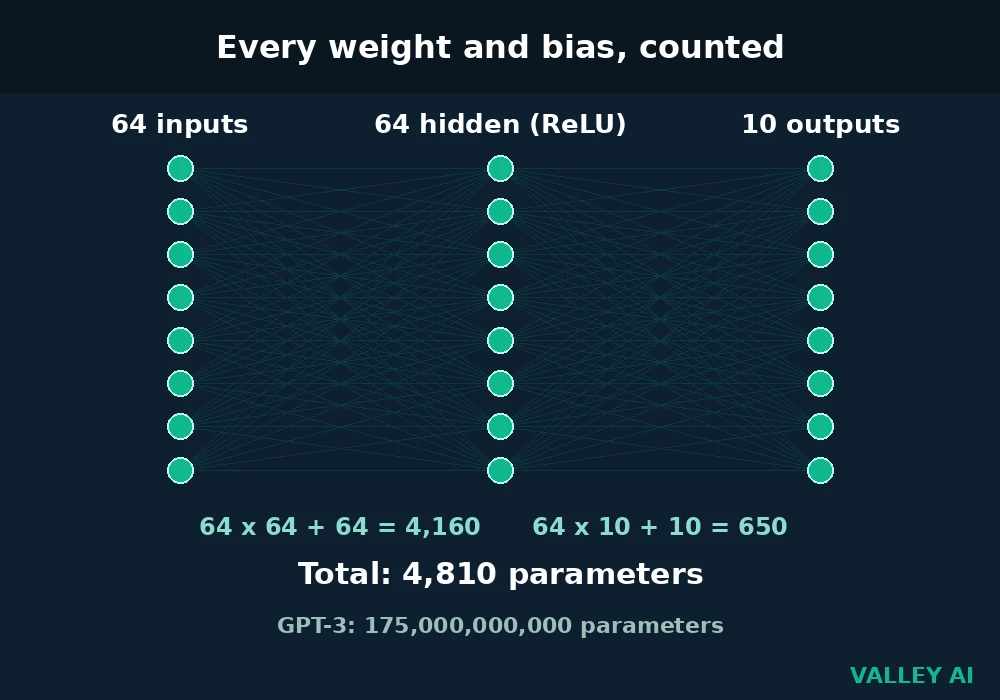
Every weight and bias is a parameter, and counting them is simple arithmetic. Multiply the number of inputs by the number of neurons, then add one bias per neuron.

Layer	Weights	Biases	Parameters
64 inputs to 64 hidden	64 x 64 = 4,096	64	4,160
64 hidden to 10 outputs	64 x 10 = 640	10	650
Total	4,736	74	4,810

Large language models follow the same arithmetic at a much bigger scale. GPT-3 holds 175 billion parameters, about 36 million times the digits network. The number matters in practice. Every parameter needs memory, needs updating during training, and needs enough examples to settle on a useful value.

Chips built to run this arithmetic fast are a separate story. A neural processing unit packs thousands of multiply-and-add units into one chip, and that is why phones can run trained networks on battery power. The same arithmetic that trains slowly on a general processor runs fast on hardware built for it.

Activation Functions Put the Bend In

The activation function decides what a neuron passes on. Four functions cover nearly every network built today.

Function	Formula	Output range	Typical use
Sigmoid	1 / (1 + e^-z)	0 to 1	Yes-or-no output
Tanh	(e^z – e^-z) / (e^z + e^-z)	-1 to 1	Hidden layers in older and recurrent networks
ReLU	max(0, z)	0 to infinity	Default choice for hidden layers
Softmax	e^zi / sum of e^zj	0 to 1, all outputs sum to 1	Multi-class output

Why does a network need an activation function at all? A neuron without one returns a weighted sum, and a stack of weighted sums is still one weighted sum. The activation bends the output, and stacked bends carve curved decision boundaries that straight lines cannot draw. Without the bend, depth adds nothing.

ReLU became the default for hidden layers because it is cheap to compute and keeps gradients from shrinking toward zero in deep stacks. It has one weakness: a neuron pushed into large negative values sticks at zero and stops learning. Variants such as Leaky ReLU give negative inputs a small slope to prevent that.

The Forward Pass: How a Prediction Is Made

A forward pass moves data from the input layer through each hidden layer to the output layer, with every neuron computing its weighted sum and activation along the way. A network where data flows in one direction only is called a feedforward network. The output layer returns one number for a yes-or-no question, one probability per class for a choice among labels, or one value for a forecast.

Engineers write each layer as a matrix multiplication, which lets graphics processors handle thousands of neurons in parallel. That is the practical reason networks train on GPUs: the arithmetic is the same operation repeated millions of times, and a GPU repeats it across thousands of cores at once.

Training and inference carry different costs, and the split matters. Training a small network is quick work on a laptop. Training a large model takes weeks on thousands of chips. Inference is the cheap half. Once training ends, only the forward pass runs, and a finished model answers in milliseconds. That split explains why a phone can run a trained network it could never train.

How a Network Learns: Loss, Backpropagation, Gradient Descent

Four steps repeat for every batch of examples until the loss stops falling.

• Forward pass: run the input through the network and get a prediction.
• Loss: measure how far the prediction sits from the correct answer.
• Backward pass: backpropagation traces the error back through the layers and works out how much each weight contributed.
• Update: gradient descent nudges every weight a small step in the direction that lowers the loss.

The loss function is the scorekeeper. For a choice among ten digits, cross-entropy is the usual measure, and random guessing scores near ln(10), which is 2.303. The digits run opened at 2.3189, almost exactly the random-guessing score, because the weights started random. Training is the climb down from that number.

How does the network know which weight to blame for an error? Backpropagation traces the error backward from the output, layer by layer, using the chain rule from calculus. A weight that pushed the prediction the wrong way gets a large gradient. A weight that barely mattered gets a small one. The 1986 paper by David Rumelhart, Geoffrey Hinton, and Ronald Williams set out the method, and it turned neural networks from a theoretical idea into something trainable.

Gradient descent uses the gradients to move the weights. Each weight steps a small amount against its gradient, and the learning rate sets the size of that step. A rate set too high overshoots the best values and the loss jumps around. A rate set too low crawls, and training takes far longer than it should. The learning rate is the one setting the network cannot tune for itself.

One full pass over the training data is an epoch. Networks train for many epochs because one pass is never enough for the weights to settle. The digits run used 200 epochs, and its loss curve tells the story of what those passes bought.

Training a Real Network: The Digits Measurement

On 8 November 2026, a small network trained on this machine with scikit-learn 1.9.1. The task was handwritten digit recognition: 1,797 images, each 8 by 8 pixels, split into 1,347 for training and 450 held back for testing. The architecture was 64 inputs, one hidden layer of 64 neurons with ReLU, and 10 outputs. Seeds were fixed, so the run repeats exactly. Training took 0.68 seconds.

Epoch	Loss	Reading
1	2.32	Random start
10	1.25	Dropping fast
50	0.17	Errors rare
200	0.03	Flattening out

The final scores were 99.78 percent on the training images and 97.78 percent on the held-back test images. The two-point gap is the number that counts. Training accuracy shows what the network memorized. Test accuracy shows what it learned.

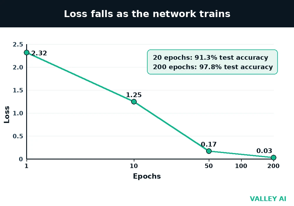
Two more runs tested the edges. The same network stopped at 20 epochs scored 91.33 percent on the test images, with a loss of 0.5428. Twenty passes were not enough, and 200 passes bought 6.5 points of test accuracy. A bigger network with 256 hidden neurons and 19,210 parameters stopped on its own at 221 passes, when the loss stopped improving, and scored 98.22 percent on the test images with 100 percent on the training images. More capacity did not hurt on this clean dataset. The extra room helped slightly, and the test score is the proof.

The 200-epoch run ended with a warning: the optimizer hit the iteration cap with the loss still falling slowly. A longer run would have pushed the loss lower, and the test score might have moved with it.

Any training run can be read through its loss curve. A steep early drop that flattens is healthy. A flat line from the start means the learning rate is too small or the data is broken. A jagged line that jumps up and down means the learning rate is too big. Read the curve before touching the architecture.

Where Neural Networks Fit, and Where They Do Not

Three designs cover most of the networks in use. Convolutional networks scan images in small patches, which suits photos and video. Recurrent networks read sequences one step at a time, and transformers read a whole sequence in parallel with attention, which is why they power modern language models.

A network is the wrong tool when the data is small. A spreadsheet of a few hundred records trains a decision tree or a logistic regression model in seconds, needs less data, and explains its answer. A network on the same data memorizes the records and fails on new ones. The simpler model wins that job.

Networks also fail loudly in one specific way: they state wrong answers with high confidence. A chatbot that invents a fact reports it with the same certainty as a true one, because the output is a probability. A high probability describes the training data. It says nothing about the world.

The test score stays the judge. A low training error means little. A low test error means the network learned something real.

Conclusion

Train one yourself. The digits run gives you the full setup: the same split, the same seeds, the same 200 epochs. Watch the loss fall and the test score climb, then change one thing, the epoch count or the hidden layer size, and watch what moves. Prediction, error, correction: that loop is the whole mechanism, and it runs the same way in a tiny network and in the largest models.

Frequently asked questions